使用Ransac进行消失点(Vanishing point )检测

Ransac

Ransac 是一种启发式的参数估计的迭代算法,在之前的一篇文章里,我也写了关于 Ransac 的相关知识,以及我自己对 Ransac 的理解。

Ransac本身并不是一个完整的可自运行的算法。 实际上,在存在离群(outliers)的情况下,它使用模型及其距离函数,鲁棒地估计模型参数。RANSAC只是在数据集上应用离群点分离,并根据最优化方法和模型的距离函数,来使用内群(inliers)估计模型参数。

因此Ransac可以完全的模块化,它允许与任何估算模型,任何距离函数和任何优化方法一起工作。从这个角度说,RANSAC也可以被认为是一种思想。

消失点(Vanishing point)

消失点(Vanishing point)是三维(3D)空间中所有平行线相交的交点。

消失点在检测道路车道方面起着重要作用,因为车道在真实世界的3D空间中是平行的,但它们在二维相机图像中车道最终会在消失点相遇。 因此,对于自动驾驶消失点检测是必要的。

以这个思想,为了检测道路,我们首先从图像中提取所有 edge 分量,然后,估计投影 edge 分量的相遇的消失点,最后,根据消失点,确定车道。

目前,消失点检测(Vanishing point detection)的算法有很多种,通过Ransac、车道纹理方向、harmony search等算法都有应用。总体而言,目前使用 Ransac 进行消失点检测最为广泛。

用于消失点检测的 Ransac 算法

Ransac 算法的基本思想可以看我之前的文章,或者参考 Wiki

基本流程如下:

  1. 建立一个拟合模型,选择拟合函数和距离函数。这里,拟合函数选择将多条线,按顺序两两寻找它们的相交点,最后取这些相交点的平均位置为我们估计的消失点位置。距离函数选择点到直线的正交距离
  2. 从线段数据集中随机采样,也为内群 ( inliers ),因为两条线相交于一点,这里我们可以选择随机采样数为2
  3. 根据随机采样的线段(数目为2),估计其相交点,即消失点的位置
  4. 计算估计的消失点到线段数据集中其他线段的距离,距离小于阈值的线段加入内群 ( inliers )
  5. 再次估计内群中的线段相交点位置,同时如第1点所述,计算模型的拟合误差
  6. 不断重复1~5,最终选择模型拟合误差最小的消失点估计位置

Python 实现

计算两直线相交点位置

我们先定义直线,两点确定一条直线

1
2
3
4
5
6
7
8
9
10
11
class Line(object):

def init(self, line):

self.x1 = line[0]

self.y1 = line[1]

self.x2 = line[2]

self.y2 = line[3]

接下来,我们计算直线的参数

对于直线方程 ax+by+c=0ax+by+c=0 ,如果我们已知直线上两点 (x1,y1)(x_1,y_1)(x2,y2)(x_2, y_2) ,那么我们可以得到直线参数:a=y1y2a = y_1-y_2b=x2x1b = x_2-x_1c=x1y2x2y1c = x_1*y_2-x_2*y_1

1
2
3
4
5
6
7
8
9
10
11
def getlineparam(line):
"""
For the line equation a*x+b*y+c=0, if we know two points(x1, y1)(x2,y2) in line, we can get
a = y1 - y2
b = x2 - x1
c = x1*y2 - x2*y1
"""
a = line.y1 - line.y2
b = line.x2 - line.x1
c = line.x1 * line.y2 - line.x2 * line.y1
return a,b,c

然后,得到了直线参数,我们计算两直线的相交点

对于两直线方程 a1x+b1y+c1=0a_1x+b_1y+c_1=0a2x+b2y+c2=0a_2x+b_2y+c_2=0 ,当 d=a1b2a2b1=0d=a_1*b_2-a_2*b_1=0 时,两直线重合或平行

相交点坐标为:

\begin{equation} \left\{\begin{matrix} x=\frac{b_1*c_2-b_2*c_1}{d}\\ y=\frac{a_2c_1-a_1c_2}{d} \end{matrix}\right. \end{equation}
1
2
3
4
5
6
7
8
9
10
11
12
13
14
15
16
def getcrosspoint(line1,line2):
"""
if we have two lines: a1*x + b1*y + c1 = 0 and a2*x + b2*y + c2 = 0,
when d(= a1 * b2 - a2 * b1) is zero, then the two lines are coincident or parallel.
The cross point is :
x = (b1 * c2 - b2 * c1) / d
y = (a2 * c1 - a1 * c2) / d
"""
a1, b1, c1 = getlineparam(line1)
a2, b2, c2 = getlineparam(line2)
d = a1 * b2 - a2 * b1
if d == 0:
return np.inf, np.inf
x = (b1 * c2 - b2 * c1) / d
y = (a2 * c1 - a1 * c2) / d
return x, y

建立消失点模型

我们需要定义一个拟合函数,以及一个距离函数

1
2
3
4
5
6
7
8
9
10
11
12
13
14
15
16
17
18
19
20
21
22
23
24
25
26
27
28
29
30
31
32
33
34
35
class pointModel(Model):
def __init__(self):
self.params = None
self.residual = 0

def fit(self, lines):
lines = lines[:,0]
X = []
Y = []

for i in range(len(lines)-1):
line1 = Line(lines[i])
line2 = Line(lines[i+1])
x, y = getcrosspoint(line1, line2)
X.append(x)
Y.append(y)

X = np.asarray(x).mean()
Y = np.asarray(y).mean()
self.params = [X, Y]

for i in range(len(lines)):
line = Line(lines[i])
a, b, c = getlineparam(line)
self.residual += abs(a*X + b*Y + c) / np.sqrt(a*a + b*b)

def distance(self, samplelines):
dists = []
for line in samplelines:
line = Line(line[0,:])
[x, y] = self.params
a, b, c = getlineparam(line)
dist = abs((a*x + b*y + c) / np.sqrt(a*a + b*b))
dists.append(dist)
return np.asarray(dists)

Ransac 算法

与之前文章的思路一致,完成Ransac代码

这里因为两条直线相交于1点,这里的min_samples建议设置为2

1
2
3
4
5
6
7
8
9
10
11
12
13
14
15
16
17
18
19
20
21
22
23
24
25
26
27
28
29
30
31
32
33
34
35
36
37
38
39
40
41
42
43
44
45
def ransac(lines, model, min_samples, min_inliers, iterations=100, eps=1, random_seed=42):
"""
Fits a model to observed data.

Uses the RANSC iterative method of fitting a model to observed data.
"""
random.seed(random_seed)

if len(lines) <= min_samples:
raise ValueError("Not enough input lines to fit the model.")

if 0 < min_inliers and min_inliers < 1:
min_inliers = int(min_inliers * len(lines))

best_params = None
best_inliers = None
best_residual = np.inf
best_iteration = None

for i in range(iterations):
indices = list(range(len(lines)))
random.shuffle(indices)
inliers = np.asarray([lines[i] for i in indices[:min_samples]])
shuffled_lines = np.asarray([lines[i] for i in indices[min_samples:]])
try:
model.fit(inliers)
dists = model.distance(shuffled_lines)
more_inliers = shuffled_lines[np.where(dists <= eps)[0]]
inliers = np.concatenate((inliers, more_inliers))

if len(inliers) >= min_inliers:
model.fit(inliers)
if model.residual < best_residual:
best_params = model.params
best_inliers = inliers
best_residual = model.residual
best_iteration = i

except ZeroDivisionError as e:
print(e)

if best_params is None:
raise ValueError("RANSAC failed to find a sufficiently good fit for the data.")
else:
return (best_params, best_inliers, best_residual, best_iteration)
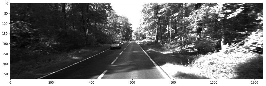
应用

我们直接处理一张车道线图片

1
2
3
4
5
6
7
8
9
import matplotlib.image as mplimg
import matplotlib.pyplot as plt
import cv2
import numpy as np
img = cv2.imread('1.png')
plt.figure(figsize=(15,5))
gray = cv2.cvtColor(img, cv2.COLOR_BGR2GRAY)
plt.imshow(gray,cmap='gray')
plt.show()
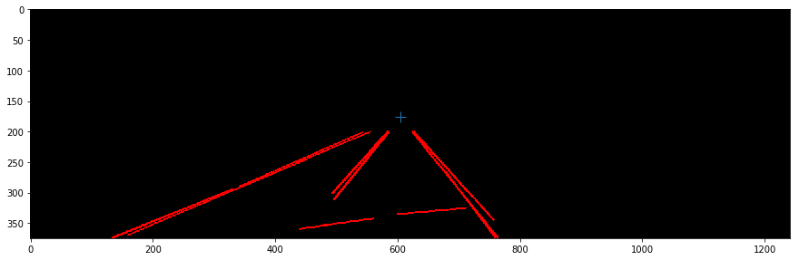
1

利用 canny edge detection 得到 edge 图,也可以选择其他滤波方法,如hat_like filter等

1
2
3
4
5
6
7
8
blur_ksize = 5  # Gaussian blur kernel size
blured = cv2.GaussianBlur(gray, (blur_ksize, blur_ksize), 0, 0)
low_threshold = 50 # Canny edge detection low threshold
high_threshold = 120 # Canny edge detection high threshold
canny = cv2.Canny(blured, low_threshold, high_threshold)
plt.figure(figsize=(15,10))
plt.imshow(canny,cmap = 'gray')
plt.show()

2

在选择出我们想要的感兴趣区域

1
2
3
4
5
6
7
8
9
10
11
12
def roi_mask(img, vertices):
mask = np.zeros_like(img)
mask_color = 255
cv2.fillPoly(mask, vertices, mask_color)
masked_img = cv2.bitwise_and(img, mask)
return masked_img

roi_vtx = np.array([[(0, img.shape[0]), (500, 200), (650, 200), (800, img.shape[0])]])
roi_edges = roi_mask(canny, roi_vtx)
plt.figure(figsize=(15,5))
plt.imshow(roi_edges, cmap='gray')
plt.show()

3

接下来用 Hough Transform 进行直线检测,关于 Hough Transform可以参考我的这篇文章

1
2
3
4
5
6
7
8
9
10
11
12
13
14
15
16
17
18
19
20
21
22
23
24
25
rho = 1
theta = np.pi / 180
threshold = 30
min_line_length = 100
max_line_gap = 20

def draw_lines(img, lines, color=[255, 0, 0], thickness=2):
for line in lines:
for x1, y1, x2, y2 in line:
cv2.line(img, (x1, y1), (x2, y2), color, thickness)

def hough_lines(img, rho, theta, threshold,
min_line_len, max_line_gap):
lines = cv2.HoughLinesP(img, rho, theta, threshold, np.array([]),
minLineLength=min_line_len,
maxLineGap=max_line_gap)
line_img = np.zeros((img.shape[0], img.shape[1], 3), dtype=np.uint8)
draw_lines(line_img, lines)
return line_img, lines


line_img, lines= hough_lines(roi_edges, rho, theta, threshold, min_line_length, max_line_gap)
plt.figure(figsize=(15,5))
plt.imshow(line_img, cmap='gray')
plt.show()

4

最后应用 Ransac 算法

1
2
3
4
5
6
Model = pointModel()
(params, inliers, residual, iteration) = ransac(lines, Model, 0.5, eps=1)
plt.figure(figsize=(15,10))
plt.imshow(line_img, cmap='gray')
plt.plot(params[0],params[1],'+', markersize=12)
plt.show()

5

效果还是很不错的!