Hat-like Filter

Introduction

在车道线检测当中，核心一步自然是的是抽取车道线的特征得到车道线检测的初步结果。实际操作中有很多方法，例如：

利用Canny算子或Sobel算子等做边缘检测
因为车道线主要是黄色或白色，可以利用不同的颜色空间（LAB、RGB、HSV等颜色空间），从颜色的值域中划分出车道线
车道线中心亮度比边缘都要高，因此可以利用 Hat-like Filter
…

以上方法大多利用车道线的低级别特征（low level feature），得到的结果需要利用Hough Transform、Ransac、sliding windows、band search等方法做进一步处理。

现在因为CNN在计算机视觉的惊人效果，所以也有人利用卷积神经网络得到 End-to-End 的车道线检测结果

利用神经网络语义分割–(SCNN)Spatial As Deep: Spatial CNN for Traffic Scene Understanding

这里主要介绍 Hat-like Filter来对车道线进行low level processing。

Hat-like Filter

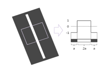
Hat-like Filter 也可以称为 Hat-shape Filter ，目的是利用车道线中心亮度比边缘都要高从鸟瞰图（bird’s view image)中过滤出我们想要的车道线[1]。车道线实际是边缘的一种，因此 Hat-like Filter 也是一种边缘检测方法。

Hat-like Filter 可以简单用下图表示：

Hat-like Filter

对于鸟瞰图像中的每个像素，计算一个特殊值 $b(x,y)$ 与其水平左右像素的值 $b(x-m,y)$ 和 $b(x + m,y)$ 进行比较，可以用如下公式表示：

$\begin{matrix} B_{+m}(x,y)=b(x,y)-b(x+m,y)\\ B_{-m}(x,y)=b(x,y)-b(x-m,y) \end{matrix}$

之后使用阈值对图像进行二值化处理：

\begin{matrix} r(x,y)=\left \{ \begin{align*} & 1, \mathrm{if}\; B_{+m} \geq 0, B_{-m} \geq 0 \;\mathrm{and} \; B_{+m}+B_{-m}\geq T\\ & 0,\mathrm{otherwise} \end{align*}\right. \end{matrix}

该边缘检测方法具有以下特性:

可以调整 $m$ 以适应不同宽度的车道线。
车道线内的像素全部标记为边缘像素，这不同于基于梯度的边缘算子（例如Sobel、Canny），可以很好地提高了车道线检测的鲁棒性
不会检测到水平边缘
对一些渐变纹理也会加强（Weighted Hat-like Filter）

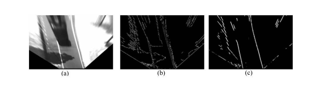
如图所示，Hat-like Filter的效果要比canny边缘检测要好。

compare

Weighted Hat-like Filter

$I_f$ ， $I_g$ 分别表示过滤后的图像和灰度图，我们将过滤器定义为[2]：

$I_f(x,y)=\delta(x,y)\cdot \left \{ 2\cdot Block_{middle}- Block_{left}-Block_{right}\right \}$

其中

$Block_{middle}= Block(x-w/2,y-h/2,w,h)$

$Block_{left}=Block(x-3w/2,y-3h/2,w,h)$

$Block_{right}=Block(x+w/2, y+h/2, w,h)$

$Block(x,y,w,h)=\sum_{(r,c)\in \left [ x,x+w \right ] \times \left [ y,y+h \right ]}{I_g(r,c)}$

这里w和h表示该块的宽度和高度。由于车道线是长条形，所以Hat-like Filter可以加强车道线区域的响应。然而，同Hat-like Filter一样，渐变纹理也被加强，这会破坏之后的二值化结果并带来许多错误检测区域。

为了克服这个问题，我们为在 $(x, y)$ 点的像素，添加一个自适应权重 $\delta(x,y)$ 。

\begin{matrix} r(x,y)=\left\{ \begin{align*} & 0, \mathrm{if} \; Block_{middle} < Block_{left}, \mathrm{or} \; Block_{middle} < Block_{right}\\ & 1,\mathrm{otherwise} \end{align*}\right. \end{matrix}

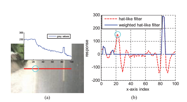
对于每个像素，如果 $Block_{middle}$ 不大于 $Block_{left}$ 或 $Block_{right}$ ，那么将会抑制此像素。因此，通过分配的权重可以显著减轻梯度纹理的影响。

如下图所示，由绿色圆圈标记的像素属于渐变纹理。使用Hat-like Filter，一些噪声的峰值被保留了下来，而我们的加权值可以显著抑制这一点。从图中还可以看出，Weighted Hat-like Filter减少了大量的错误检测。之后进行二值化等进一步操作。

Weighted Hat-like Filter

两个方向一起过滤的 Weighted Hat-like Filter

这里注意到[2]中的 Weighted Hat-like Filter 是一个方向的，我们可以通过加入与另一个方向的与and 操作，这样的效果会更加明显。

Python实现并比较

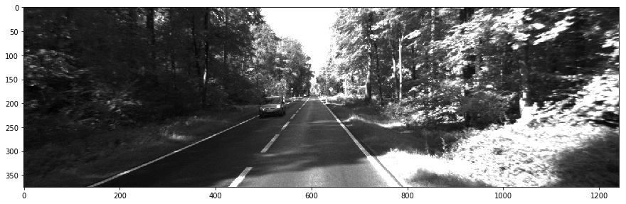
加载图片，并转为灰度图

import matplotlib.image as mplimg
import matplotlib.pyplot as plt
import cv2
import numpy as np
img = cv2.imread('1.png')
gray = cv2.cvtColor(img, cv2.COLOR_BGR2GRAY)
plt.figure(figsize=(15,10))
plt.imshow(gray,cmap='gray')
plt.show()

original

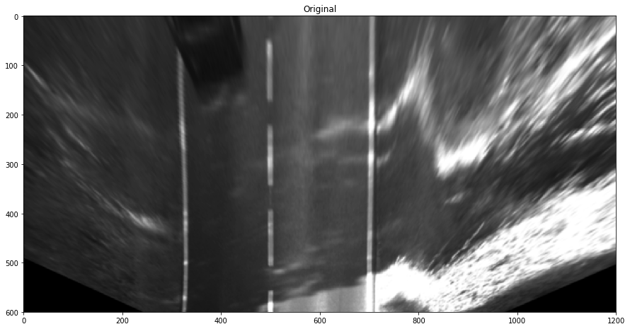
利用IPM，计算出转换矩阵，并将图片转为鸟瞰图（Bird’s view image)

img_size = (1200, 600)
blur_ksize = 5
src = np.float32([[435, 375],[775, 375],[500, 300],[710, 300]])
dst = np.float32([[500, 600],[700, 600],[500, 500],[700, 500]])
M = cv2.getPerspectiveTransform(src, dst)
warped = cv2.warpPerspective(gray, M, img_size)
warped = cv2.GaussianBlur(warped, (blur_ksize, blur_ksize), 0, 0)
plt.figure(figsize=(15,10))
plt.title('Original')
plt.imshow(warped,cmap='gray')
plt.show()

Bird's view

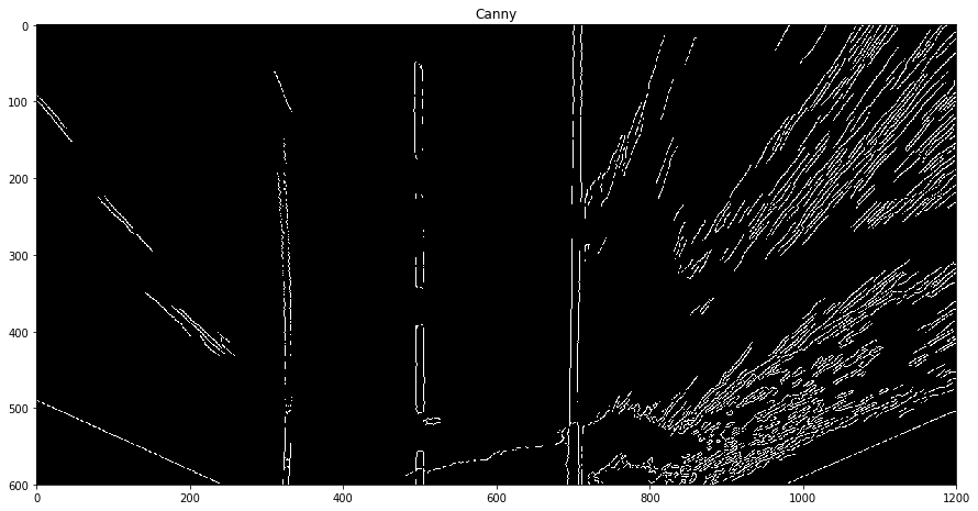
Canny边缘检测

low_threshold = 50 # Canny edge detection low threshold
high_threshold = 120  # Canny edge detection high threshold
canny = cv2.Canny(warped, low_threshold, high_threshold)
plt.figure(figsize=(15,10))
plt.title('Canny')
plt.imshow(canny,cmap = 'gray')
plt.show()

Canny

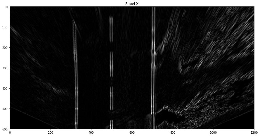
Sobel算子，这里使用的是x方向

sobelx = cv2.Sobel(warped,cv2.CV_16S,1,0,ksize=5)
sobely = cv2.Sobel(warped,cv2.CV_16S,0,1,ksize=5)

sobelx = np.absolute(sobelx)
sobely = np.absolute(sobely)

plt.figure(figsize=(15,10))
plt.imshow(sobelx,cmap = 'gray')
plt.title('Sobel X')
plt.show()

Sobel

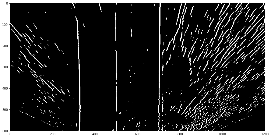
Hat-like Filter

这里实现的比较繁琐，已经经过了二值化处理

def hat_like(img, m, T):
    left_mat = np.ones((1, m)) * -1
    right_mat = np.ones((1, m)) * -1
    center_mat = np.ones((1, m))

    conv_mat1 = np.column_stack((left_mat, center_mat, np.zeros((1, m))))
    conv_mat2 = np.column_stack((np.zeros((1, m)), center_mat, right_mat))
    conv1 = cv2.filter2D(img, cv2.CV_16S, conv_mat1)
    conv2 = cv2.filter2D(img, cv2.CV_16S, conv_mat2)
    conv1[conv1<0]=0
    conv2[conv2<0]=0
    
    res = np.logical_and(conv1,conv2)
    
    conv_mat3 = np.column_stack((left_mat, center_mat*2, right_mat))
    conv3 = cv2.filter2D(img, cv2.CV_16S, conv_mat3)
    conv3[conv3<T]=0
    
    res = np.logical_and(res,conv3)
    res[res<0]=0
    return res

plt.figure(figsize=(15,10))
plt.imshow(hat_like_conv_y(warped, 5, 50), cmap='gray')
plt.show()

Hat-like Filter

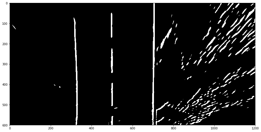
Weighted Hat-like Filter

因为车道线检测中，对于图片边缘是可以忽视的，这里没有对图片边缘的卷积做太多处理。

def weighted_hat_like_conv(img, w, h, T):
    left_upper_mat = np.ones((h, w)) * -1
    right_bottom_mat = np.ones((h, w)) * -1
    center_mat = np.ones((h, w)) * 2

    top = np.column_stack((left_upper_mat, np.zeros((h,w*2))))
    middle = np.column_stack((np.zeros((h,w)), center_mat, np.zeros((h, w))))
    bottom = np.column_stack((np.zeros((h,w*2)), right_bottom_mat))

    conv_mat = np.row_stack((top, middle, bottom))
    res = cv2.filter2D(img, cv2.CV_16S, conv_mat)
    
    res[res<=T] = 0
    res[res>T] = 1
    return res

plt.figure(figsize=(15,10))
plt.imshow(weighted_hat_like_conv(warped, 7, 3, 1000), cmap='gray')
plt.show()

Weighted Hat-like Filter

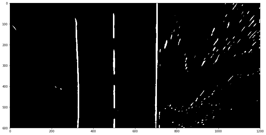
两方向相与的Weighted Hat-like Filter

def weighted_hat_like_conv_and(img, w, h, T):
    left_upper_mat = np.ones((h, w)) * -1
    right_bottom_mat = np.ones((h, w)) * -1
    center_mat = np.ones((h, w)) * 2

    top = np.column_stack((left_upper_mat, np.zeros((h,w*2))))
    middle = np.column_stack((np.zeros((h,w)), center_mat, np.zeros((h, w))))
    bottom = np.column_stack((np.zeros((h,w*2)), right_bottom_mat))

    conv_mat1 = np.row_stack((top, middle, bottom))
    conv_mat2 = np.row_stack((bottom, middle, top))
    
    res1 = cv2.filter2D(img, cv2.CV_16S, conv_mat1)
    res1[res1 < T] = 0
    res2 = cv2.filter2D(img, cv2.CV_16S, conv_mat2)
    res2[res2 < T] = 0

    #res = np.bitwise_and(res1, res2)
    res = np.logical_and(res1, res2)
    return res

plt.figure(figsize=(15,10))
plt.imshow(weighted_hat_like_conv_and(warped, 7, 3, 1000), cmap='gray')
plt.show()

and

Reference

[1] R. Jiang, M. Terauchi, R. Klette, S. Wang, and T. Vaudrey, “Low-Level Image Processing for Lane Detection and Tracking,” in Arts and Technology, vol. 30, F. Huang and R.-C. Wang, Eds. Berlin, Heidelberg: Springer Berlin Heidelberg, 2010, pp. 190–197.

[2] Bei He, Rui Ai, Yang Yan, and Xianpeng Lang, “Accurate and robust lane detection based on Dual-View Convolutional Neutral Network,” 2016, pp. 1041–1046.

目录

Introduction

Hat-like Filter

Weighted Hat-like Filter

两个方向一起过滤的 Weighted Hat-like Filter

Python实现并比较

Reference