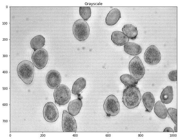
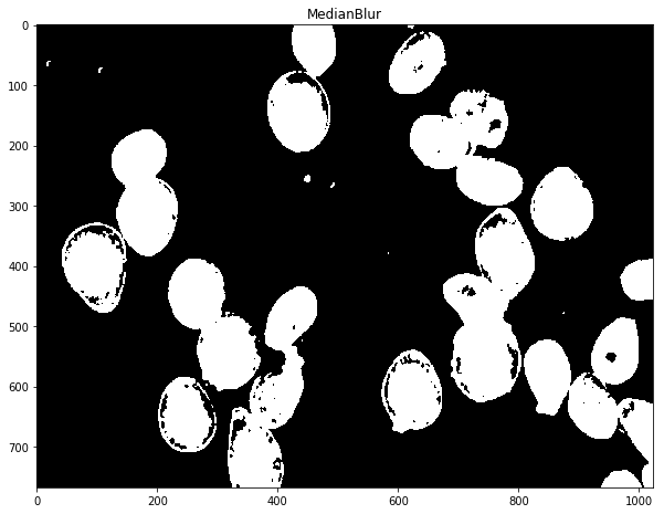
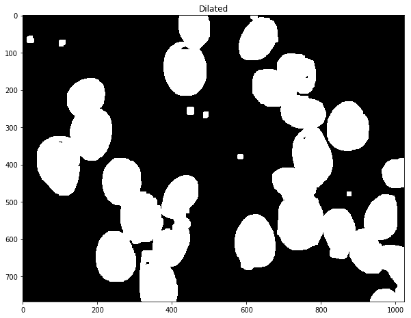
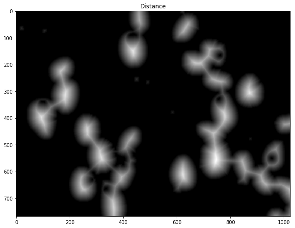
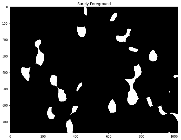
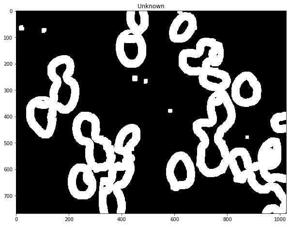
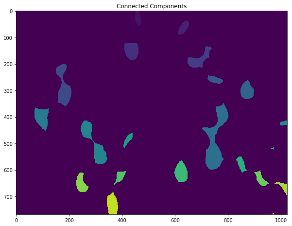
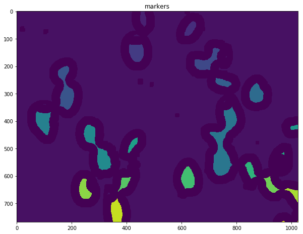
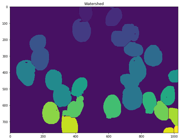
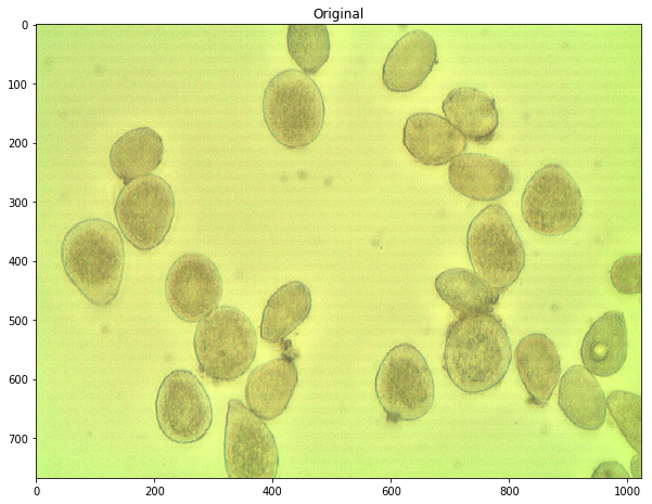
这是在Stackoverflow上发现的一个通过图像处理计算细胞的例子,里面利用了很多基础的算法,Ostu、Watershed等,是一个很不错的学习的文章。

原文地址:点此

问题

从微观样本中计算一种疾病的孢子数量,但到目前为止还没有取得多大成功。因为孢子的颜色与背景相似,而且许多都很接近。
图片如下所示:

fungus spores

解决的思路和方法

一般来说,针对这种分离近距离或接触斑点或物体的问题,我们可以使用分水岭方法(Watershed),同时也可以找一些论文,来帮助我们研究这样的问题,如:Detection and Segmentation of Multiple Touching Product Inspection Items

这里沿着Stackoverflow里的思路,我们来尝试解决这个问题

步骤和Python代码

首先,我们准备一些辅助代码,帮助我们显示图片

1
2
3
4
5
6
7
8
9
10
11
12
13
14
15
16
17
18
19
20
21
import numpy as np
import cv2
import matplotlib.pyplot as plt
from skimage.morphology import watershed as skwater

def showImage(title, img, ctype):
plt.figure(figsize=(10,10))
if ctype == "bgr":
rgb = cv2.cvtColor(img,cv2.COLOR_BGR2RGB)
plt.imshow(rgb)
elif ctype == "hsv":
hsv = cv2.cvtColor(img,cv2.COLOR_HSV2RGB)
plt.imshow(hsv)
elif ctype == "gray":
plt.imshow(img, cmap="gray")
elif ctype == "rgb":
plt.imshow(img)
else:
raise Exception("Unknown color type.")
plt.title(title)
plt.show()

下图就是我们的原始图像

1
2
img = cv2.imread("cell.jpg")
showImage("Original", img, "bgr")

png

Otsu方法是一种自适应阈值化方法,可以用来分割颜色。一般来说,该方法假设可以将图像的像素强度绘制成双峰的直方图,找到灰度直方图的一个最佳的分离点,并以此找到该图的二值化阈值。采取的具体方法为两个部分的类间方差最大,也可以转化为两个部分的类内方差最小。

(而对于假设为单峰的灰度直方图的图像,我们可以采用triangle方法来进行自适应阈值化。)

接下来我们用Ostu方法对图片做自适应阈值化

1
2
3
4
gray = cv2.cvtColor(img, cv2.COLOR_BGR2GRAY)
ret, thresh = cv2.threshold(gray, 0, 255, cv2.THRESH_BINARY_INV+cv2.THRESH_OTSU)
showImage("Grayscale", gray, "gray")
showImage("Applying Otsu", thresh, "gray")

png

png

我们可以看到在图片里有很多的白色的噪声,并且在细胞的内部也出现了一些黑色的斑点,对于前者中值滤波是一个简单有效的办法,对于后者,我们可以使用dilate。
(这里也可以通过闭运算、开运算以及其他滤波方法来移除这些噪声,还可以通过计算区域面积来去除小区域,以及利用区域生长的方法来填充孔洞并去除小区域)

1
2
3
4
5
6
median = cv2.medianBlur(thresh, 5)
showImage('MedianBlur', median, 'gray')

kernel = np.ones((3, 3), np.uint8)
dilated = cv2.dilate(median, kernel, iterations=5)
showImage('Dilated',dilated,'gray')

png

png

我们现在需要确定分水岭(watershed)的峰值并给它们单独的标签。

为此,执行距离变换,然后过滤掉距离单元中心太远的距离。

1
2
dist = cv2.distanceTransform(dilated, cv2.DIST_L2, 5)
showImage('Distance',dist,'gray')

png

1
2
3
fraction_foreground = 0.5
ret, sure_fg = cv2.threshold(dist,fraction_foreground*dist.max(),255,0)
showImage('Surely Foreground',sure_fg,'gray')

png

上述图像中的每个白色区域是单独的单元。

现在我们通过减去最大值来识别未知区域,即由分水岭算法标记的区域:

1
2
unknown = cv2.subtract(dilated,sure_fg.astype(np.uint8))
showImage('Unknown',unknown,'gray')

png

未知区域应在每个细胞周围形成一个的甜甜圈样子的圆环。

接下来,我们给出距离变换唯一标签产生的每个不同区域,然后在最终执行分水岭变换之前标记未知区域:

1
2
3
4
5
6
7
8
9
10
11
12
13
14
15
16
# Marker labelling
ret, markers = cv2.connectedComponents(sure_fg.astype(np.uint8))
showImage('Connected Components',markers,'rgb')

# Add one to all labels so that sure background is not 0, but 1
markers = markers+1

# Now, mark the region of unknown with zero
markers[unknown == np.max(unknown)] = 0

showImage('markers',markers,'rgb')

dist = cv2.distanceTransform(dilated,cv2.DIST_L2,5)
markers = skwater(-dist,markers,watershed_line=True)

showImage('Watershed',markers,'rgb')

png

png

png

现在,细胞的总数为标记的数量减去1(为了忽略背景):

这下再看看我们的原始图片。

1
showImage("Original", img, "bgr")

png

1
len(set(markers.flatten()))-1
23

可以通过调整距离阈值,dilation的程度或者使用h-maxima(局部阈值最大值)来使得结果变得更准确。

但要注意过度拟合; 也就是说,调整单个图像得到的最好结果,对其他图片可能并不起效果。

估计不确定性

还可以通过略微修改参数,以了解计数中的不确定性。

1
2
3
4
5
6
7
8
9
10
11
12
13
14
15
16
17
18
19
20
21
22
23
24
25
26
27
28
29
30
31
32
33
34
35
36
37
38
39
import itertools

def CountCells(dilation=5, fg_frac=0.6):
#Read in image
img = cv2.imread('cell.jpg')
#Convert to a single, grayscale channel
gray = cv2.cvtColor(img,cv2.COLOR_BGR2GRAY)
#Threshold the image to binary using Otsu's method
ret, thresh = cv2.threshold(gray,0,255,cv2.THRESH_BINARY_INV+cv2.THRESH_OTSU)
#Adjust iterations until desired result is achieved
kernel = np.ones((3,3),np.uint8)
dilated = cv2.dilate(thresh, kernel, iterations=dilation)
#Calculate distance transformation
dist = cv2.distanceTransform(dilated,cv2.DIST_L2,5)
#Adjust this parameter until desired separation occurs
fraction_foreground = fg_frac
ret, sure_fg = cv2.threshold(dist,fraction_foreground*dist.max(),255,0)
# Finding unknown region
unknown = cv2.subtract(dilated,sure_fg.astype(np.uint8))
# Marker labelling
ret, markers = cv2.connectedComponents(sure_fg.astype(np.uint8))
# Add one to all labels so that sure background is not 0, but 1
markers = markers+1
# Now, mark the region of unknown with zero
markers[unknown==np.max(unknown)] = 0
markers = skwater(-dist,markers,watershed_line=True)
return len(set(markers.flatten()))-1

#Smaller numbers are noisier, which leads to many small blobs that get
#thresholded out (undercounting); larger numbers result in possibly fewer blobs,
#which can also cause undercounting.
dilations = [4,5,6]
#Small numbers equal less separation, so undercounting; larger numbers equal
#more separation or drop-outs. This can lead to over-counting initially, but
#rapidly to under-counting.
fracs = [0.5, 0.6, 0.7, 0.8]

for params in itertools.product(dilations,fracs):
print("Dilation={0}, FG frac={1}, Count={2}".format(*params,CountCells(*params)))
Dilation=4, FG frac=0.5, Count=22
Dilation=4, FG frac=0.6, Count=23
Dilation=4, FG frac=0.7, Count=17
Dilation=4, FG frac=0.8, Count=12
Dilation=5, FG frac=0.5, Count=21
Dilation=5, FG frac=0.6, Count=23
Dilation=5, FG frac=0.7, Count=20
Dilation=5, FG frac=0.8, Count=13
Dilation=6, FG frac=0.5, Count=20
Dilation=6, FG frac=0.6, Count=23
Dilation=6, FG frac=0.7, Count=24
Dilation=6, FG frac=0.8, Count=14

最后针对这些数字做一些统计学上的数据处理,来得到我们想要的结果

Reference

Stackoverflow: Improve accuracy of image processing to count fungus spores